Activation Functions in Neural Networks
Activation functions are a crucial component of artificial neural networks, serving as the mathematical operation that determines the output of a node or neuron. They introduce non-linearities to the network, allowing it to learn complex patterns and relationships within the data.
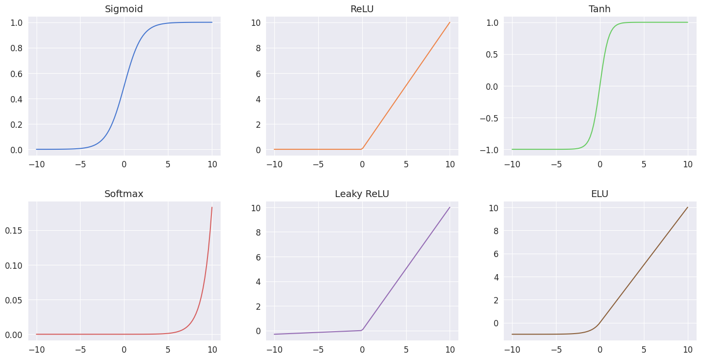
1. Sigmoid Function
Sigmoid function, also known as the logistic function. This function squashes input values between 0 and 1, making it a popular choice for the output layer in binary classification problems. Here’s what it looks like mathematically:
$$ \sigma(x) = \frac{1}{1 + e^{-x}} $$
And in Python:
import numpy as np

def sigmoid(x):
    return 1 / (1 + np.exp(-x))
2. ReLU (Rectified Linear Unit)
ReLU is one of the most popular activation functions in deep learning. It replaces all negative values in the input with zero, while leaving positive values unchanged.
Mathematically, the ReLU function is defined as:
$$ f(x) = \max(0, x) $$
def relu(x):
    return np.maximum(0, x)
3. Tanh Function
Tanh (Hyperbolic Tangent) is like the sigmoid function’s cooler, more balanced sibling. It squashes input values between -1 and 1, offering a symmetric range of outputs.
Mathematically, the tanh function is defined as:
$$ \text{tanh}(x) = \frac{e^x - e^{-x}}{e^{x + e^{-x}}}$$
def tanh(x):
    return np.tanh(x)
4. Softmax Function
When you’re dealing with multi-class classification problems, the softmax function is the one you want to call. This function converts raw scores into probabilities, ensuring that the sum of all probabilities equals 1.
Mathematically, the softmax function is defined as:
$$ \text{softmax}(x_i) = \frac{e^{x_i}}{\sum_{j} e^{x_j}} $$
def softmax(x):
    exp_x = np.exp(x - np.max(x))  # For numerical stability
    return exp_x / np.sum(exp_x, axis=0)
5. Leaky ReLU
Leaky ReLU is like ReLU’s rebellious cousin. Instead of shutting down completely for negative inputs, it allows a small, non-zero gradient to flow through. This helps to address the dreaded “dying ReLU” problem, keeping the party going even when things get a little negative.
Mathematically, the leaky ReLU function is defined as:
$$ f(x) = \begin{cases} x & \text{if } x > 0 \ \alpha x & \text{otherwise} \end{cases} $$
def leaky_relu(x, alpha=0.01):
    return np.where(x > 0, x, alpha * x)
6. ELU (Exponential Linear Unit)
The ELU activation function is like the cool kid on the block, combining the best of both worlds – the robustness of ReLU and the ability to capture negative values. It’s a smooth, continuous function that avoids the “dying ReLU” problem while still providing the beneficial properties of ReLU.
Mathematically, the ELU function is defined as:
$$ f(x) = \begin{cases} x & \text{if } x > 0 \ \alpha (e^{x} - 1) & \text{otherwise} \end{cases} $$
And in Python:
import numpy as np

def elu(x, alpha=1.0):
    return np.where(x > 0, x, alpha * (np.exp(x) - 1))
These are just a few examples of activation functions used in neural networks. Each activation function has its advantages and disadvantages, and the choice often depends on the specific problem being solved and empirical performance on validation data. Experimentation with different activation functions is crucial to finding the most suitable one for your neural network architecture and dataset.
Loss Functions in Machine Learning
Alright, now that we’ve had our fun with activation functions, let’s talk about loss functions, also known as cost functions or objective functions. These Functions are the ones that measure the difference between our model’s predictions and the actual values, quantifying its performance and guiding the optimization process.
Mean Squared Error (MSE)
- Calculates the average squared difference between predicted and actual values.
- Commonly used in regression problems.
- Mathematically: $$ MSE = \frac{1}{n} \sum_{i=1}^{n} (y_i - \hat{y}_i)^2 $$
Binary Cross-Entropy Loss
- Used in binary classification problems to measure the dissimilarity between predicted probabilities and actual binary labels.
- Mathematically: $$ BCE = -\frac{1}{n} \sum_{i=1}^{n} [y_i \log(\hat{y}_i) + (1 - y_i) \log(1 - \hat{y}_i)] $$
Categorical Cross-Entropy Loss
- An extension of binary cross-entropy loss for multi-class classification problems.
- Measures the dissimilarity between predicted class probabilities and one-hot encoded target labels.
- Mathematically: $$ CCE = -\frac{1}{n} \sum*{i=1}^{n} \sum*{j=1}^{m} y*{ij} \log(\hat{y}*{ij}) $$
Hinge Loss (for SVM)
- Used in support vector machines (SVM) for binary classification.
- Penalizes misclassified examples based on their distance from the decision boundary.
- Mathematically: $$ HingeLoss = \max(0, 1 - y_i \cdot \hat{y}_i) $$
Huber Loss
- Combines the advantages of squared error loss and absolute error loss.
- Less sensitive to outliers compared to MSE.
- Mathematically: $$ HuberLoss = \begin{cases} \frac{1}{2}(y - \hat{y})^2 & \text{if } |y - \hat{y}| \leq \delta \ \delta(|y - \hat{y}| - \frac{1}{2}\delta) & \text{otherwise} \end{cases} $$
Custom Loss Functions
- In some cases, you might need to roll up your sleeves and craft your own custom loss functions tailored to your specific problem requirements.
- Just make sure these functions are differentiable to facilitate gradient-based optimization.
Loss functions are selected based on the nature of the problem, the type of output, and the desired properties of the model’s predictions. Choosing an appropriate loss function is crucial for achieving optimal performance and training stability.